!pip install numpy matplotlib jax scipy scikit-optimize ucimlrepo optax

import numpy as np
import matplotlib.pyplot as plt
import cvxpy as cp
import jax
from jax import numpy as jnp, grad
from scipy.optimize import minimize_scalar
import jax.numpy as jnp
from jax import grad, jit, hessian
from sklearn.model_selection import train_test_split
from sklearn.preprocessing import StandardScaler
import time
from ucimlrepo import fetch_ucirepo
from optax.losses import safe_softmax_cross_entropy as cros_entr
from sklearn.preprocessing import StandardScaler
from scipy.optimize import minimize_scalar
import sklearn.datasets as skldata

# Set a random seed for reproducibility
np.random.seed(228)
jax.random.PRNGKey(228)

Array([  0, 228], dtype=uint32)

@jit
def logistic_loss(w, X, y, mu=1):
    m, n = X.shape
    return jnp.sum(jnp.logaddexp(0, -y * (X @ w))) / m + mu / 2 * jnp.sum(w**2)

def generate_problem(m=1000, n=300, mu=1):
    X, y = skldata.make_classification(n_classes=2, n_features=n, n_samples=m, n_informative=n//2, random_state=0)
    X = jnp.array(X)
    y = jnp.array(y)

    X_train, X_test, y_train, y_test = train_test_split(X, y, test_size=0.33, random_state=42)

    return X_train, y_train, X_test, y_test

def compute_optimal(X, y, mu):
    w = cp.Variable(X.shape[1])
    objective = cp.Minimize(cp.sum(cp.logistic(cp.multiply(-y, X @ w))) / len(y) + mu / 2 * cp.norm(w, 2)**2)
    problem = cp.Problem(objective)
    problem.solve()
    return w.value, problem.value

@jit
def compute_accuracy(w, X, y):
    # Compute predicted probabilities using the logistic (sigmoid) function
    preds_probs = jax.nn.sigmoid(X @ w)
    # Convert probabilities to class predictions: -1 if p < 0.5, else 1
    preds = jnp.where(preds_probs < 0.5, 0, 1)
    # Calculate accuracy as the average of correct predictions
    accuracy = jnp.mean(preds == y)
    return accuracy



# @jit
def compute_metrics(trajectory, x_star, f_star, times, X_train, y_train, X_test, y_test, mu):
    f = lambda w: logistic_loss(w, X_train, y_train, mu)
    metrics = {
        "f_gap": [jnp.abs(f(x) - f_star) for x in trajectory],
        "x_gap": [jnp.linalg.norm(x - x_star) for x in trajectory],
        "time": times,
        "train_acc": [compute_accuracy(x, X_train, y_train) for x in trajectory],
        "test_acc": [compute_accuracy(x, X_test, y_test) for x in trajectory],
    }
    return metrics

def gradient_descent(w_0, X, y, learning_rate=0.01, num_iters=100, mu=0):
    trajectory = [w_0]
    times = [0]
    w = w_0
    f = lambda w: logistic_loss(w, X, y, mu)
    iter_start = time.time()
    for i in range(num_iters):
        grad_val = grad(f)(w)
        if learning_rate == "linesearch":
            # Simple line search implementation
            phi = lambda alpha: f(w - alpha*grad_val)
            result = minimize_scalar(fun=phi, 
                                     bounds=(1e-3, 2e2)
                              )
            step_size = result.x
        else:
            step_size = learning_rate
        w -= step_size * grad_val
        iter_time = time.time()
        trajectory.append(w)
        times.append(iter_time - iter_start)
    return trajectory, times

def run_experiments(params):
    mu = params["mu"]
    m, n = params["m"], params["n"]
    methods = params["methods"]
    results = {}

    X_train, y_train, X_test, y_test = generate_problem(m, n, mu)
    n_features = X_train.shape[1]  # Number of features
    params["n_features"] = n_features
    
    x_0 = jax.random.normal(jax.random.PRNGKey(0), (n_features, ))
    x_star, f_star = compute_optimal(X_train, y_train, mu)

    for method in methods:
        learning_rate = method["learning_rate"]
        iterations = method["iterations"]
        trajectory, times = gradient_descent(x_0, X_train, y_train, learning_rate, iterations, mu)
        label = method["method"] + " " + str(learning_rate)
        results[label] = compute_metrics(trajectory, x_star, f_star, times, X_train, y_train, X_test, y_test, mu)

    return results, params

def plot_results(results, params):
    plt.figure(figsize=(11, 5))
    mu = params["mu"]
    
    if mu > 1e-2:
        plt.suptitle(f"Strongly convex binary logistic regression. mu={mu}.")
    else:
        plt.suptitle(f"Convex binary logistic regression. mu={mu}.")

    plt.subplot(2, 4, 1)
    for method, metrics in results.items():
        plt.plot(metrics['f_gap'])
    plt.xlabel('Iteration')
    plt.ylabel(r'$|f(x) -f^*|$')
    plt.yscale('log')
    plt.grid(linestyle=":")

    plt.subplot(2, 4, 2)
    for method, metrics in results.items():
        plt.plot(metrics['x_gap'], label=method)
    plt.xlabel('Iteration')
    plt.ylabel('$\|x_k - x^*\|$')
    plt.yscale('log')
    plt.grid(linestyle=":")

    plt.subplot(2, 4, 3)
    for method, metrics in results.items():
        plt.plot(metrics["train_acc"])
    plt.xlabel('Iteration')
    plt.ylabel('Train accuracy')
    # plt.yscale('log')
    plt.grid(linestyle=":")

    plt.subplot(2, 4, 4)
    for method, metrics in results.items():
        plt.plot(metrics["test_acc"])
    plt.xlabel('Iteration')
    plt.ylabel('Test accuracy')
    # plt.yscale('log')
    plt.grid(linestyle=":")

    plt.subplot(2, 4, 5)
    for method, metrics in results.items():
        plt.plot(metrics["time"], metrics['f_gap'])
    plt.xlabel('Time')
    plt.ylabel(r'$|f(x) -f^*|$')
    plt.yscale('log')
    plt.grid(linestyle=":")

    plt.subplot(2, 4, 6)
    for method, metrics in results.items():
        plt.plot(metrics["time"], metrics['x_gap'])
    plt.xlabel('Time')
    plt.ylabel('$\|x_k - x^*\|$')
    plt.yscale('log')
    plt.grid(linestyle=":")

    plt.subplot(2, 4, 7)
    for method, metrics in results.items():
        plt.plot(metrics["time"], metrics["train_acc"])
    plt.xlabel('Time')
    plt.ylabel('Train accuracy')
    # plt.yscale('log')
    plt.grid(linestyle=":")

    plt.subplot(2, 4, 8)
    for method, metrics in results.items():
        plt.plot(metrics["time"], metrics["test_acc"])
    plt.xlabel('Time')
    plt.ylabel('Test accuracy')
    # plt.yscale('log')
    plt.grid(linestyle=":")

    # Place the legend below the plots
    plt.figlegend(loc='lower center', ncol=5, bbox_to_anchor=(0.5, -0.00))
    # Adjust layout to make space for the legend below
    filename = ""
    for method, metrics in results.items():
        filename += method
    filename += f"_{mu}.pdf"
    plt.tight_layout(rect=[0, 0.05, 1, 1])
    plt.savefig(filename)
    plt.show()

<>:133: SyntaxWarning: invalid escape sequence '\|'
<>:165: SyntaxWarning: invalid escape sequence '\|'
<>:133: SyntaxWarning: invalid escape sequence '\|'
<>:165: SyntaxWarning: invalid escape sequence '\|'
/var/folders/6l/qhfv4nh50cqfd22s2mp1shlm0000gn/T/ipykernel_87087/2871042674.py:133: SyntaxWarning: invalid escape sequence '\|'
  plt.ylabel('$\|x_k - x^*\|$')
/var/folders/6l/qhfv4nh50cqfd22s2mp1shlm0000gn/T/ipykernel_87087/2871042674.py:165: SyntaxWarning: invalid escape sequence '\|'
  plt.ylabel('$\|x_k - x^*\|$')

params = {
    "mu": 0,
    "m": 1000,
    "n": 100,
    "methods": [
        {
            "method": "GD",
            "learning_rate": 3e-1,
            "iterations": 2000,
        },
        {
            "method": "GD",
            "learning_rate": 7e-1,
            "iterations": 2000,
        },
    ]
}

results, params = run_experiments(params)
plot_results(results, params)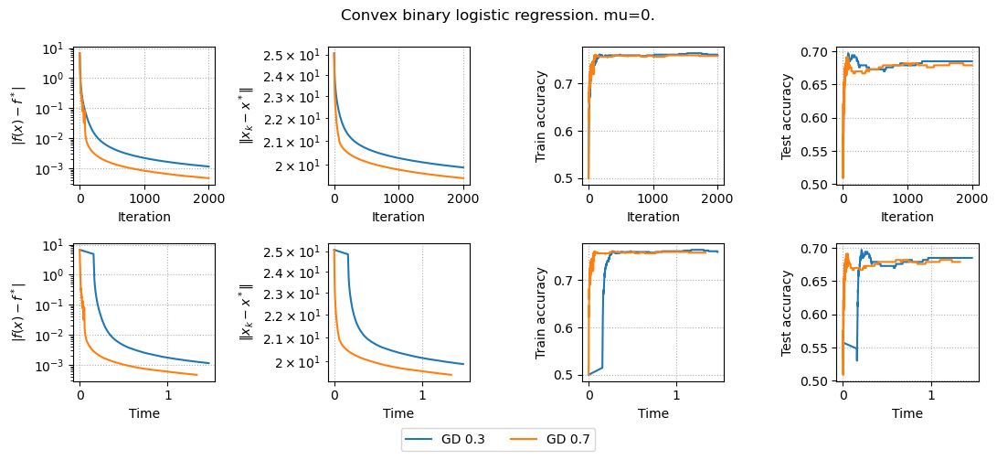

params = {
    "mu": 1e-1,
    "m": 1000,
    "n": 100,
    "methods": [
        {
            "method": "GD",
            "learning_rate": 1e-1,
            "iterations": 900,
        },
        {
            "method": "GD",
            "learning_rate": 1.1e-1,
            "iterations": 900,
        },
    ]
}

results, params = run_experiments(params)
plot_results(results, params)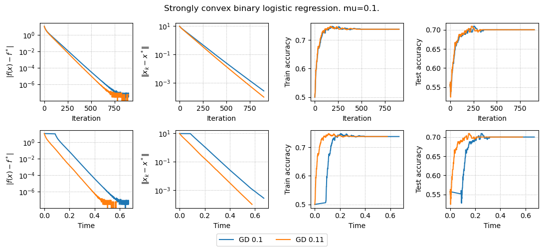

Now we also have convergence in terms of distance to the solution, but it does not influence accuracy.

Support Vector Machine

import numpy as np
import matplotlib.pyplot as plt
import cvxpy as cp
import jax
from jax import numpy as jnp, grad
from scipy.optimize import minimize_scalar
import jax.numpy as jnp
from jax import grad, jit, hessian
from sklearn.model_selection import train_test_split
from sklearn.preprocessing import StandardScaler
import time
from ucimlrepo import fetch_ucirepo
from optax.losses import safe_softmax_cross_entropy as cros_entr
from sklearn.preprocessing import StandardScaler
from scipy.optimize import minimize_scalar
import sklearn.datasets as skldata

# Set a random seed for reproducibility
np.random.seed(228)
jax.random.PRNGKey(228)

Array([  0, 228], dtype=uint32)

# Set a random seed for reproducibility
np.random.seed(228)
jax.random.PRNGKey(228)

# Generate a synthetic binary classification dataset
def generate_svm_data(m=1000, n=300):
    X, y = skldata.make_classification(n_classes=2, n_features=n, n_samples=m, 
                                       n_informative=n//2, random_state=42)
    y = 2 * y - 1  # Convert labels to {-1, 1}
    return X, y

# Solve SVM using convex optimization
def compute_svm_optimal(X, y, C=1.0):
    m, n = X.shape
    w = cp.Variable(n)
    b = cp.Variable()
    slack = cp.Variable(m)

    # SVM objective: minimize 1/2 ||w||^2 + C * sum(slack)
    objective = cp.Minimize(0.5 * cp.norm(w, 2)**2 + C * cp.sum(slack))

    # Constraints:  y_i (x_i^T w + b) >= 1 - slack_i,  slack_i >= 0
    constraints = [
        cp.multiply(y, X @ w + b) >= 1 - slack,
        slack >= 0
    ]

    problem = cp.Problem(objective, constraints)
    problem.solve()

    return w.value, b.value, problem.value

# Hinge loss function
@jax.jit
def hinge_loss(w, b, X, y, C=1.0):
    margins = y * (X @ w + b)
    loss = jnp.maximum(0, 1 - margins)
    return 0.5 * jnp.sum(w**2) + C * jnp.mean(loss)

# Compute accuracy
@jax.jit
def compute_accuracy(w, b, X, y):
    preds = jnp.sign(X @ w + b)
    return jnp.mean(preds == y)

# Perform gradient descent for SVM optimization
def gradient_descent_svm(w_0, b_0, X, y, learning_rate=0.01, num_iters=100, C=1.0):
    trajectory = [w_0]
    times = [0]
    w, b = w_0, b_0
    f = lambda w, b: hinge_loss(w, b, X, y, C)
    
    iter_start = time.time()
    for i in range(num_iters):
        grad_w, grad_b = grad(f, argnums=(0, 1))(w, b)
        w -= learning_rate * grad_w
        b -= learning_rate * grad_b

        iter_time = time.time()
        trajectory.append(w)
        times.append(iter_time - iter_start)
    
    return trajectory, times

# Run SVM Experiments
def run_experiments_svm(params):
    C = params["C"]
    m, n = params["m"], params["n"]
    methods = params["methods"]
    results = {}

    X, y = generate_svm_data(m, n)
    X_train, X_test, y_train, y_test = train_test_split(X, y, test_size=0.33, random_state=42)
    
    # Standardize data
    scaler = StandardScaler()
    X_train = scaler.fit_transform(X_train)
    X_test = scaler.transform(X_test)

    w_0 = jax.random.normal(jax.random.PRNGKey(0), (n,))
    b_0 = 0.0

    w_star, b_star, f_star = compute_svm_optimal(X_train, y_train, C)

    for method in methods:
        learning_rate = method["learning_rate"]
        iterations = method["iterations"]
        trajectory, times = gradient_descent_svm(w_0, b_0, X_train, y_train, learning_rate, iterations, C)
        label = method["method"] + " " + str(learning_rate)
        results[label] = {
            "f_gap": [jnp.abs(hinge_loss(w, b_0, X_train, y_train, C) - f_star) for w in trajectory],
            "x_gap": [jnp.linalg.norm(w - w_star) for w in trajectory],
            "time": times,
            "train_acc": [compute_accuracy(w, b_0, X_train, y_train) for w in trajectory],
            "test_acc": [compute_accuracy(w, b_0, X_test, y_test) for w in trajectory],
        }

    return results, params

# Plot Results
def plot_results_svm(results, params):
    plt.figure(figsize=(11, 5))
    C = params["C"]
    
    plt.suptitle(f"SVM Training Results. C={C}")

    plt.subplot(2, 4, 1)
    for method, metrics in results.items():
        plt.plot(metrics['f_gap'])
    plt.xlabel('Iteration')
    plt.ylabel(r'$|f(x) -f^*|$')
    plt.yscale('log')
    plt.grid(linestyle=":")

    plt.subplot(2, 4, 2)
    for method, metrics in results.items():
        plt.plot(metrics['x_gap'], label=method)
    plt.xlabel('Iteration')
    plt.ylabel('$\|x_k - x^*\|$')
    plt.yscale('log')
    plt.grid(linestyle=":")

    plt.subplot(2, 4, 3)
    for method, metrics in results.items():
        plt.plot(metrics["train_acc"])
    plt.xlabel('Iteration')
    plt.ylabel('Train accuracy')
    plt.grid(linestyle=":")

    plt.subplot(2, 4, 4)
    for method, metrics in results.items():
        plt.plot(metrics["test_acc"])
    plt.xlabel('Iteration')
    plt.ylabel('Test accuracy')
    plt.grid(linestyle=":")

    plt.subplot(2, 4, 5)
    for method, metrics in results.items():
        plt.plot(metrics["time"], metrics['f_gap'])
    plt.xlabel('Time')
    plt.ylabel(r'$|f(x) -f^*|$')
    plt.yscale('log')
    plt.grid(linestyle=":")

    plt.subplot(2, 4, 6)
    for method, metrics in results.items():
        plt.plot(metrics["time"], metrics['x_gap'])
    plt.xlabel('Time')
    plt.ylabel('$\|x_k - x^*\|$')
    plt.yscale('log')
    plt.grid(linestyle=":")

    plt.subplot(2, 4, 7)
    for method, metrics in results.items():
        plt.plot(metrics["time"], metrics["train_acc"])
    plt.xlabel('Time')
    plt.ylabel('Train accuracy')
    plt.grid(linestyle=":")

    plt.subplot(2, 4, 8)
    for method, metrics in results.items():
        plt.plot(metrics["time"], metrics["test_acc"])
    plt.xlabel('Time')
    plt.ylabel('Test accuracy')
    plt.grid(linestyle=":")

    plt.figlegend(loc='lower center', ncol=5, bbox_to_anchor=(0.5, -0.00))
    plt.tight_layout(rect=[0, 0.05, 1, 1])
    plt.show()

<>:119: SyntaxWarning: invalid escape sequence '\|'
<>:149: SyntaxWarning: invalid escape sequence '\|'
<>:119: SyntaxWarning: invalid escape sequence '\|'
<>:149: SyntaxWarning: invalid escape sequence '\|'
/var/folders/6l/qhfv4nh50cqfd22s2mp1shlm0000gn/T/ipykernel_86548/3657982053.py:119: SyntaxWarning: invalid escape sequence '\|'
  plt.ylabel('$\|x_k - x^*\|$')
/var/folders/6l/qhfv4nh50cqfd22s2mp1shlm0000gn/T/ipykernel_86548/3657982053.py:149: SyntaxWarning: invalid escape sequence '\|'
  plt.ylabel('$\|x_k - x^*\|$')

params = {
    "C": 0,
    "m": 1000,
    "n": 100,
    "methods": [
        {
            "method": "GD",
            "learning_rate": 3e-3,
            "iterations": 2000,
        },
        {
            "method": "GD",
            "learning_rate": 7e-3,
            "iterations": 2000,
        },
    ]
}

results, params = run_experiments_svm(params)
plot_results_svm(results, params)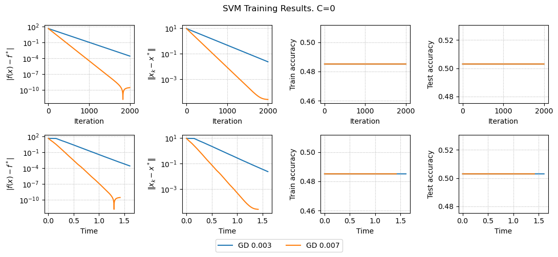

Here we only minimize \frac{1}{2} ||w||_2^2 without hinge loss, we have linear convergence both for function error and distance to the solution.

params = {
    "C": 0.1,
    "m": 1000,
    "n": 100,
    "methods": [
        {
            "method": "GD",
            "learning_rate": 3e-3,
            "iterations": 2000,
        },
        {
            "method": "GD",
            "learning_rate": 7e-3,
            "iterations": 2000,
        },
    ]
}

results, params = run_experiments_svm(params)
plot_results_svm(results, params)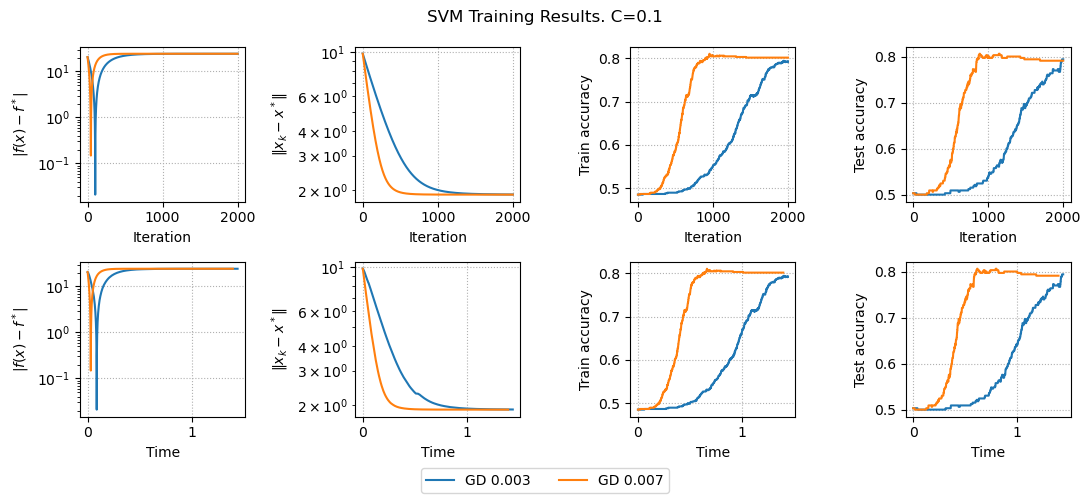

Here we minimize regularized hinge loss and see that we have accuracy improvement.